Heuristics Hit Different: Speed-Boosting Your Path-Finding

Have you faced a problem so large that checking every possible solution is nearly impossible? Consider planning a road trip across many cities or organizing a complex schedule. These problems involve countless combinations. Traditional algorithms often settle too quickly on solutions that seem good but are far from optimal.

Simulated Annealing (SA) offers a smarter approach. Inspired by metallurgy, it explores many solutions at first, accepting worse options early. As the temperature drops, the algorithm becomes more selective, refining the solution toward optimality.

Why Simulated Annealing Works

To understand why Simulated Annealing is such a powerful tool, it helps to look at the problem it solves better than most traditional optimization methods.  Many algorithms try to find the best solution by always moving in the direction of improvement. At first, this approach sounds effective.

However, it has a major limitation. The algorithm can easily get stuck in a local optimum. This is a solution that appears optimal within a small neighborhood but is far from the best possible overall solution.

Escaping Local Optima Through Controlled Randomness

Imagine climbing hills in thick fog, trying to reach the highest peak. A greedy algorithm will always move up when it can. It stops when there’s no higher hill. If it ends up on a small hill, it believes it has reached the top.

Simulated Annealing avoids this pitfall. At the start, it’s bold and willing to move downhill. This temporary loss is part of the strategy, allowing the algorithm to explore other areas and potentially find the true peak.

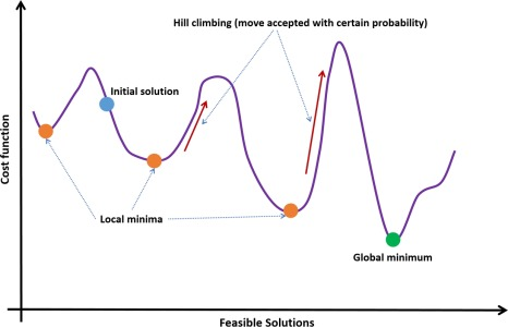
Simulated Annealing procedure (blue (mid gray in print version) dot – initial solution, orange (light gray in print version) dot – local minimum, green (mid gray in print version) dot – global minimum, red (dark gray in print version) arrow – hill climbing (move accepted with certain probability)).

This idea is driven by a fundamental principle: controlled randomness. Instead of behaving rigidly from the start, Simulated Annealing introduces a variable called temperature, that controls how willing the algorithm is to accept worse solutions.

At the beginning of the process, the temperature is set high. This means the algorithm is deliberately tolerant of mistakes:

• It embraces experimentation, 
• Tries risky moves, 
• Explores distant possibilities and, 
• Accepts solutions that are technically worse than the current one. 

This may feel counterintuitive, but that initial flexibility is exactly what allows Simulated Annealing to escape rigid thinking and avoid getting trapped in shallow local optima.

As the temperature gradually decreases, this tolerance fades. The algorithm becomes more selective, accepting fewer and fewer worse moves, and slowly transitions from exploration into refinement. By the end, only genuine improvements are considered, guiding the solution into a stable and refined state. 

The Maths Behind Simulated Annealing Decisions

Another reason SA works is the mathematical foundation behind those decisions. When a worse solution appears, the algorithm doesn’t just flip a coin. Its chance of acceptance follows a precise probability function based on the difference between solutions and the current temperature. The poorer the new solution, the less likely it is to be accepted. The cooler the environment becomes, the stricter the acceptance rule turns. This balance between exploration and exploitation allows SA to stretch farther than many classical methods, without losing direction. Mathematically, the acceptance probability can be expressed as:

P(accept)=e-ET

Where 

• E=Enew-Ecurrent, is the increase in cost (or energy)
• T is the temperature

This formula has deep meaning:

• If the new solution is only slightly worse (E small), it is likely to be accepted.
• If the new solution is much worse (E large), it is rarely accepted.
• If the temperature T is high, even bad solutions are often accepted.
• If T is low, almost no bad solutions are accepted.

So temperature directly controls how adventurous the algorithm is. The temperature is gradually reduced according to a cooling schedule, typically something like: 

Tk+1​=αTk with 0<α<1

This exponential decay slowly transforms the algorithm from an explorer into a refiner.

• Early phase: high T, high randomness → exploration.
• Late phase: low T, low randomness → convergence.

This dynamic shift is what prevents premature convergence while still guaranteeing stabilization. SA generates a Markov Chain whose stationary distribution at temperature T is 

π(x) ∝  e-E(x)T, As T0

This distribution becomes increasingly concentrated around the global minima of E(x). In other words, the algorithm becomes statistically biased toward optimal solutions as it cools.

Finally, Simulated Annealing works because it mirrors the real behavior of physical systems. In metallurgy, slow cooling lets atoms settle into highly ordered structures instead of chaotic ones. By imitating this process computationally, we benefit from millions of years of natural optimization.

In practice, Simulated Annealing can explore enormous solution spaces and still find solutions close to the best possible, even when millions or billions of combinations exist. It transforms randomness into strategy, and uncertainty into structure. That’s why, decades after its invention, it remains a favorite across diverse fields—from engineering and logistics to AI and science.

A Practical Example: Traveling Salesperson Problem

Given N cities (points), find the shortest tour that visits each city once and returns to start.

• State S: a permutation (ordering) of cities
• Energy E(S): total tour length
• Neighbor move: a 2-opt swap (reverse a segment) — standard TSP move that’s simple and strong.

Representing the problem

Cities

We store cities as 2D points: points = [(x1, y1), (x2, y2), …]. Each city is just a coordinate.

A “tour” (a solution)

A tour is a permutation of city indices: tour = [0, 5, 2, 1, 4, …]

Meaning: visit city 0 → then city 5 → then city 2 → … and finally return to the start.

This representation is super common because it’s simple and it guarantees you visit each city exactly once.

Measuring quality: the cost function

Distance between two cities

def distance(a, b):

    return math.hypot(a[0] – b[0], a[1] – b[1])

math.hypot(dx, dy) 

Computes the euclidean distance between both cities through Pythagoras theorem.

Total tour length (energy)

def tour_length(points, tour):

    total = 0.0

    n = len(tour)

    for i in range(n):

        total += distance(points[tour[i]], points[tour[(i + 1) % n]])

    return total

Key detail: (i + 1) % n wraps around so the last city connects back to the first city, forming a loop. This tour_length is your energy E(S) in SA terms.

Generating a neighbor: the 2-opt move

To explore the search space, SA needs to propose “nearby” solutions.

def two_opt_neighbor(tour):

    n = len(tour)

    i, j = sorted(random.sample(range(n), 2))

    new_tour = tour[:]

    new_tour[i:j+1] = reversed(new_tour[i:j+1])

    return new_tour

What this does:

• pick two random indices i < j
• reverse the subsegment from i to j

This is called 2-opt and it’s great for TSP because it can remove crossings, makes structural changes and it’s still cheap to compute.

Example:

Tour: [0, 1, 2, 3, 4, 5]
If i=2, j=4, reverse [2,3,4] → [4,3,2]

New tour: [0, 1, 4, 3, 2, 5]

The Simulated Annealing loop

This is the heart of it:

current = shuffled tour

best = current

curr_E = tour_length(current)

best_E = curr_E

T = T0

Now repeat for many iterations the following steps:

Step 1: propose a candidate solution

candidate = two_opt_neighbor(current)

cand_E = tour_length(candidate)

dE = cand_E – curr_E

dE <= 0 means the candidate is better (shorter tour), meanwhile dE > 0 means worse.

Step 2: accept or reject with Metropolis criterion

if dE <= 0 or random.random() < math.exp(-dE / T):

    current = candidate

    curr_E = cand_E

If it’s better: take it. If it’s worse: maybe take it depending on temperature.

The probability of accepting worse moves is P(accept)=e-ET, as said at the very beginning of this article. So:

• early (high T): accepts worse moves often → exploration
• late (low T): almost never accepts worse moves → refinement

Step 3: track the best-ever solution

if curr_E < best_E:

    best = current[:]

    best_E = curr_E

Even if the search later wanders, we keep the best solution found so far.

Step 4: cool down

T *= alpha, this makes the algorithm gradually more strict.

Final Results

The four figures illustrate how Simulated Annealing transforms a random, inefficient solution into a structured and near-optimal one. The first plot shows the initial tour, which is a random ordering of cities. The path jumps chaotically across the plane, producing many long crossings and unnecessary detours. This results in a very large total distance (around 18.8 in this run). This is typical: a random solution contains no structure and therefore serves as a good baseline to demonstrate improvement. The temperature curve shows a rapid initial drop followed by a long, slow tail.

• Early on, temperature is relatively high, so the algorithm frequently accepts worse moves.
• This allows the search to move freely and escape bad local structures.
• As temperature decreases, acceptance of worse moves becomes rarer, and the algorithm gradually stabilizes.

By about 1000 iterations, the temperature is already close to zero, meaning the algorithm is effectively behaving like a greedy local optimizer from that point onward.

The cost curve reveals the core dynamic of Simulated Annealing:

• The steep drop at the beginning corresponds to rapid structural improvements in the tour.
• The small upward spikes represent moments where worse solutions were accepted temporarily.
• The long flat region at the end shows convergence: the algorithm is no longer exploring and is only making very small refinements.

This pattern — rapid improvement, noisy exploration, and slow stabilization — is exactly the behavior Simulated Annealing is designed to produce.

The final tour has a total length of about 4.9, compared to the initial 18.8 — a dramatic improvement. The structure is visibly smoother: fewer crossings, shorter jumps, and a more natural geometric progression through the points. While not guaranteed to be globally optimal, the result is already very close to the best possible for this random instance as you can see in this Github code.

Conclusion: From Intuition to Intelligence

What makes Simulated Annealing especially valuable is its generality. It requires no gradients, no convexity assumptions, and no special structure beyond the ability to compare solutions and generate neighbors. This makes it applicable to a wide range of problems — from scheduling and routing to machine learning and game AI — where traditional optimization techniques struggle.

In the end, Simulated Annealing teaches a broader lesson about problem solving: sometimes, progress does not come from always making the best possible move, but from allowing temporary setbacks in service of deeper exploration. By embracing uncertainty early and discipline later, the algorithm turns randomness into structure and complexity into tractability.